This week’s report: Trends radar: October 2–8, 2026 — 226 clusters from 12,788 stories, and 6 topics where the LLM analyst disagreed with the numbers.
The Disagreement
The first real run of the weekly pipeline finished on July 16th. The quantitative side of the system had embedded 900 recent articles, grouped them into 395 clusters, counted each cluster week by week, and then stamped a status on the 8 that qualified.
One of those clusters was a set of articles about evaluating AI systems. The math called it “fading” with a z-score of −0.18 and growth of 0.85× compared to its recent average. That’s a pretty clear verdict. The topic had a soft week and was on its way out.
Then the LLM analyst read the same numbers and overruled it:
The quantitative layer calls this cluster “fading” based on a z-score of –0.18, but the underlying articles span Gradient Flow and Eugene Yan and cover three distinct sub-arguments: evaluation is the real bottleneck (not model quality), AI operational bills are rising even as token prices fall, and agents need to be judged on task completion rather than capability demos. That is a coherent, durable storyline rather than a single viral piece decaying. Flagging as Emerging in the ledger rather than fading…
That wasn’t a bug, and it wasn’t the LLM going off the rails either. The system is designed so the two halves can contradict each other. Every disagreement is recorded with a reason, and the weekly report has a section just for exploring the disagreements. Neither layer gets the final word.
Two months and ten weekly runs later, “AI Systems Evaluation & Operational Cost” is still on the analyst’s ledger as Emerging. One soft week wasn’t decay after all.
This post covers why I built it that way, the three things that went wrong along the way, and what each of them taught me. There’s a prompt at the end if you want to build one for your own data.
When you combine classical ML and LLM reasoning, don’t blend them. Oppose them, and make the disagreement easy to inspect.
What I Wanted
I curate Data Elixir, so I read a lot of what gets published about data and AI. I already have a system called DistillWorks that answers “what’s good today?” What I didn’t have was something that answers a different question: what’s moving? What’s showing up more this month than last month, what’s brand new, and what’s quietly going away?
That’s a trends question, and trends are about time. A single great article isn’t a trend. Twenty people writing about the same thing over three weeks might be.
So I built TrendsWorks. It runs locally on my laptop, uses the same directory-as-agent setup as my investing assistant, and sends me a report every Friday to help prep the newsletter.
The Shape of It
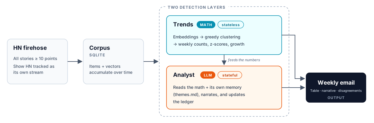
Items come in every day and pile up in a SQLite database. Once a week, two very different layers look at that pile:
- The math layer is stateless. It embeds items, clusters them, counts each cluster by week, and applies a fixed rule that labels each one either new, emerging, accelerating, fading, or steady. It re-derives everything from scratch on every run and remembers nothing. The only place an LLM touches this layer is to give a name to clusters that already qualified on the numbers.
- The analyst layer is stateful. A single LLM call reads the math’s output along with its own memory, which is a markdown file of themes it’s been tracking. It writes the narrative, updates that file, and lists every place where it disagrees with the math.
That’s the whole contract. The analyst is responsible for carrying storylines across weeks, and the math is responsible for the numbers. The analyst can argue with the numbers but can’t change them.
Here’s what a disagreement looks like in the output. This one is from last week’s run, where the analyst noticed that a cluster’s label didn’t match what was in it:
{
  "subject": "Apple App Store policies and developer disputes (34 items, emerging, z 3.33)",
  "math_says": "A sizeable emerging cluster labeled around App Store policy and developer disputes.",
  "analyst_says": "Mostly a mislabeled Apple hardware-launch spike — the exemplars are iPhone 18 Pro, AirPods 5, Mac mini M6, iPhone Duo, not policy disputes.",
  "why": "The cluster label doesn't describe its contents; the mass is a September Apple-event product dump (a predictable calendar spike), with only one genuine App-Store-rejection item, so the 'developer disputes' framing overstates a real trend."
}The math has no memory. The LLM has no authority over the numbers. Each one is strong exactly where the other is blind.
It took a few wrong turns to get to that point.
Failure #1: One Cluster Called “Everything AI”
My first clustering run used a cosine similarity threshold of 0.75, which is a pretty standard starting point. It produced one giant cluster of 351 items. That was about a third of the corpus, and it included LLM evals, cyberattack dashboards, and AI billing, all lumped together.
The problem was that I trusted a threshold before I’d measured the space it was operating in. So I ran a quick test on two sentences that have nothing to do with each other:
from shared.embeddings import embed_texts

a, b = embed_texts([
    "DuckDB adds columnar json support",
    "A recipe for sourdough bread",
])
print(a @ b)   # 0.595
Databases and sourdough came out at 0.595. With this embedding model (gemini-embedding-001), unrelated text sits around 0.6. A 0.75 threshold is barely above noise, which is why nearly anything with “AI” in it ended up in the same bucket.
So I swept the threshold across a range of values:
| threshold | clusters | largest | singleton rate |
|---|---|---|---|
| 0.75 | 15 | 351 | 40% |
| 0.80 | 101 | 243 | 66% |
| 0.83 | 248 | 94 | 71% |
| 0.85 | 395 | 69 | 77% |
| 0.88 | 590 | 33 | 83% |
The numbers alone don’t tell you which row is right. For that, I wrote a small script that prints the contents of each cluster at a given threshold, and then I just read them. At 0.85, the clusters snapped into single topics: Bayesian bandits, PostgreSQL internals, approximate nearest neighbors. At 0.88, related articles started splitting apart.
There’s no metric here. The evaluation is me reading clusters and deciding whether they belong together. At this scale, that’s fine. A human who knows the domain can look at 30 clusters in ten minutes and tell whether they’re coherent, and that’s a better check than any metric I could have set up.
This came up again later. Titles alone turned out to be thin, so I changed what gets embedded. Now it’s the title plus the top comments, which say a lot more about what a story is actually about. I re-ran the calibration after that change. The best threshold was still 0.85, but the clusters at that threshold were a lot better. The big catch-all blob split into several coherent themes. Same number, different input, and I only knew it still held because I checked.
Embedding spaces have geometry. Thresholds don’t transfer between models, or even between different inputs on the same model. Calibration is something you measure, not a default you inherit.
Failure #2: Blogs Don’t Trend
With clustering fixed, the first run’s strongest signal (z = 1.36, growth 3.14×) turned out to be… one prolific author writing about PostgreSQL. Great posts, but one person publishing on their own schedule isn’t a trend. The analyst spent a big chunk of that first report explaining why single-source clusters don’t count.
The next strongest signals were two clusters built entirely from one vendor’s product blog. The analyst threw those out too:
These are product release notes, not trend signal. A vendor announcing GreyNoise integration or SOC 2 certification does not constitute a community storyline.
It was right, and the problem wasn’t the model. It was the data. At that point, the corpus was mostly RSS feeds from about 200 blogs. Blogs are great context, but trends need many independent people reacting to the same things, with real timestamps. A feed of 200 personal blogs is 200 sample sizes of one.
So I switched the main source to the Hacker News firehose and pulled every story that gets at least 10 points, which works out to about 150 a day. I also dropped the keyword filtering.
The original version of the HN agent searched for keywords like “pandas,” “sql,” and “machine learning.” That seems sensible, but it means the system could only ever find things I already knew to look for. If I’m building a system to judge quality, filtering for precision makes sense. For a radar, I want coverage. My filters were encoding my blind spots.
Hacker News also has a practical advantage: Algolia indexes all of it, with timestamps, going back years. I backfilled 12 months of history in minutes. The corpus went from about 4,300 mostly-blog items to over 57,000 today, including nearly 3,900 Show HN posts.
Before tuning a model, ask whether your data can even contain the answer. And watch your filters, because they encode your blind spots.
Failure #3: Time Is a Schema Decision
This one is less dramatic but it’s the gotcha most people will hit.
Hacker News has a memory. I can ask Algolia for everything posted last March and get it back with real timestamps. RSS doesn’t. A feed shows you what’s in it right now, and once a post scrolls off the end, it’s gone for good. That’s why the system keeps its own corpus. If you can’t go back and get a source’s history, you have to collect it as it happens.
Once you’re collecting, you need a clock. Every item gets a discovered_at timestamp the first time the system sees it, and that value never changes. If the same story shows up the next day with more points, only the engagement numbers get updated.
That sounds like a small detail, but if re-seeing an item bumped its timestamp, every popular story would smear across several weeks and the weekly counts would lie. discovered_at is the trend clock, and the whole math layer depends on it being honest.
Then the backfill nearly broke it. Backfilled items need discovered_at set to the story’s original published time. If you naively stamp them with “now,” a year of history collapses into a single day. Worse, in my case it also tripped a sanity rule meant to catch RSS feeds that resurface ancient posts. Neither failure is obvious until you look at a histogram with one enormous bar in it.
There’s one more time rule worth mentioning: the math only analyzes complete weeks. The report goes out Friday morning and covers Friday through Thursday night. The in-progress week is excluded, so the system never mistakes “the week isn’t over yet” for “this trend is dying.”
Every timestamp in a schema is a claim about what time means. Decide which clock measures the thing you care about, then protect it with rules that can’t be broken by accident.
Why I Kept It Boring
There are two choices here that people will want to argue with, so let me get ahead of them.
No vector database. Embeddings are stored as BLOBs in SQLite. The pipeline never does live nearest-neighbor lookups. It clusters one window, once a week, in one batch, and brute-force cosine similarity over the whole thing is a few milliseconds of numpy at this scale. A vector database would be more infrastructure to run for a search problem this system doesn’t have.
No HDBSCAN. The clustering is a greedy centroid algorithm in about 40 lines. It has one knob, the threshold from Failure #1, and every assignment has a one-sentence explanation: “this item was at least 0.85 similar to that cluster’s centroid.” Here’s the whole thing:
def cluster_items(vectors: np.ndarray, threshold: float = 0.75) -> list[Cluster]:
    """Assign each vector (rows L2-normalized, chronological order) to the
    most similar existing cluster if cosine ≥ threshold, else start a new
    one. Returns clusters ordered by first appearance."""
    clusters: list[Cluster] = []
    if len(vectors) == 0:
        return clusters
    centroids = np.empty((0, vectors.shape[1]), dtype=np.float32)
    sums = np.empty((0, vectors.shape[1]), dtype=np.float32)  # unnormalized member sums

    for i, vec in enumerate(vectors):
        if len(clusters) > 0:
            sims = centroids @ vec
            best = int(np.argmax(sims))
            if sims[best] >= threshold:
                clusters[best].member_indices.append(i)
                sums[best] += vec
                c = sums[best] / np.linalg.norm(sums[best])
                centroids[best] = c
                clusters[best].centroid = c
                continue
        # start a new cluster
        clusters.append(Cluster(centroid=vec.copy(), member_indices=[i]))
        centroids = np.vstack([centroids, vec[None, :]])
        sums = np.vstack([sums, vec[None, :]])

    return clusters
A fancier algorithm could probably produce slightly better clusters, but the whole point of this system is that the analyst (and I) can argue with the math, and you can’t argue with something you can’t explain.
Legibility is a feature you can design for. In a system whose job is to be argued with, it’s the feature everything else rests on.
Where the LLMs Actually Are
It’s easy to assume a system like this is LLM calls all the way down. It isn’t:
| call | model tier | volume | cost |
|---|---|---|---|
| embeddings | commodity embedding model | ~150 items/day (backfill once) | pennies; ~$1–2 for the whole year |
| cluster labels | cheapest chat tier (Haiku) | ~40 tiny calls/week | cents |
| the analyst | frontier tier (Opus) | 1 call/week | ~$0.25 |
Getting items into the system is completely mechanical. No LLM decides what to fetch or what’s relevant. The funnel narrows before the expensive judgment happens, not after. By the time the analyst runs, it’s reading a compact summary of maybe a few dozen clusters, not tens of thousands of articles.
Early on, I was on the free tier for embeddings, which capped me at 1,000 requests a day. I had a backlog of more than 50,000 items, so at that rate it would have taken almost two months to catch up.
The fix was to embed newest first. The weekly analysis only looks at the last few weeks, so that part filled in within a day or two and the deep history caught up on its own. When you’re rationed, the order you spend the quota in matters as much as how much you have.
Use the best model for the one call that actually requires judgment, and keep everything around it mechanical. What an LLM system costs to run is a design decision, not a bill you discover later.
The Memory Is a Markdown File
All of the analyst’s memory across weeks lives in one file, themes.md. Each theme gets a status, when it was first seen, a summary, evidence, and a “watch for” line. Here’s the entry the analyst wrote for the AI evaluation theme on that first run:
## AI Systems Evaluation & Operational Cost
**Status:** Emerging
**First seen:** 2026-07-16
**Last updated:** 2026-07-16
**Summary:** A growing body of practitioner writing argues that evaluation
quality and inference cost management — not model capability — are the real
bottlenecks for AI in production. The conversation spans LLM evals, agent
task-completion benchmarks, and the paradox of rising AI bills even as
per-token prices fall.
**Evidence:** Gradient Flow published at least five pieces in the 12-week
window on this theme ('Generation is cheap. Evaluation is everything.', 'Your
AI agent looks capable. But can it actually finish the job?', 'Why your AI
bills are going up even as tokens get cheaper'). Eugene Yan's 'How to Work and
Compound with AI' adds a practitioner workflow angle. Consistent weekly
presence across the full window.
**Watch for:** New tooling announcements around LLM evaluation frameworks
(e.g., updates to LangSmith, RAGAS, or new entrants); cost-benchmarking posts
from cloud providers or infra startups; whether the agent-reliability angle
spawns its own cluster.
I like the “watch for” line a lot. It’s the analyst leaving a note for its future self about what would confirm or kill the theme. On the next run, when no standalone cluster showed up for it, it added: “If it stays invisible in the math for another 2–3 runs, reconsider status.” That’s the kind of judgment a z-score can’t make.
The analyst rewrites this file every week, but anything I add by hand under a theme survives the rewrite. So if I think it’s wrong about something, I can say so right there in its own memory, and it’ll read my note next Friday.
Just like with the investing assistant, I didn’t need a database for this. A markdown file is easy to read, easy to edit, and easy to put in git.
Agent memory should be readable, editable, and hard to lose. A markdown file that you and the model can both write to does all three.
What the Argument Buys You
Going back to that first run, the analyst’s override only carries weight because the math’s verdict is printed right next to it. If I’d let the LLM quietly adjust the status, I’d have a system that sounds smart and can’t be checked. If I’d only trusted the math, I’d have thrown out a real theme after one slow week.
Neither layer is the ground truth. The tension between them is the product.
It keeps working, too. Last week the math flagged a brand-new cluster about a UN vote on world map projections: z-score 6.91, growth 14×. The analyst called it what it was, one news moment and out of scope. In the same report, it took an AI-and-mathematics cluster that the math just called “emerging,” connected it to two quiet weeks and a new research-integrity angle it had been tracking in its ledger, and upgraded the theme to Accelerating. The math couldn’t see that trajectory. The analyst couldn’t have found the cluster without the math.
And when they agree, that’s a signal too. The disagreements section never gets dropped from the email. If there’s nothing to report, it says “None this week — the layers agree.”
The corpus now holds a full year of Show HN, every builder launch with at least 10 points, clustered and trended. What that shows about what people are building is its own post, coming soon.
Prompt
If you’re interested in playing with these ideas, here’s a prompt to get started with. Your data will be different from mine, and most of the lessons in this post came from questions about the data, not the model. So the prompt starts with an interview instead of a spec. It covers the four questions that shaped every design decision here. Your answers will be different from mine, and that’s the point.
This is also exactly how TrendsWorks started: an interview about sources, what “trend” should mean, and when the report is needed, all before any code got written.
Show the prompt
I want to build a trends radar over a stream of text — something that
detects what's *moving* over time, not just what's new today. Before
writing any code, interview me:

1. **The stream.** What text arrives over time that I care about?
   (forum posts, support tickets, papers, reviews, commit messages,
   news…) For whatever I name, press me on three properties: Does it
   carry honest timestamps? Can history be backfilled, or does the
   corpus only start the day we turn it on? And is it many independent
   voices reacting to the same world — which can trend — or a few
   voices on their own schedules, which is context, not signal?
2. **The decision.** What decision or ritual will the report feed, and
   when does it happen? The time-bucket boundary and delivery day
   should serve that moment, not the calendar.
3. **What "trend" means to me.** Rising volume? Acceleration? Things
   appearing from nothing? Things fading? Which of those would I
   actually act on?
4. **What the model will actually see.** For each item, what text
   genuinely describes what it's *about*? Titles? Bodies? Replies?
   Make me verify the input isn't boilerplate before we embed anything.

Then propose a design that follows these principles — and tell me where
my situation justifies breaking them:

- **Two deliberately contrasting layers.** A stateless quantitative
  layer (embed → cluster → count per complete time bucket →
  deterministic status rules) that re-derives everything each run, and
  an LLM analyst with a human-editable memory file that interprets the
  numbers, carries storylines across windows, and must list every
  disagreement with the math. Disagreements are surfaced, never
  auto-reconciled.
- **A persistent corpus** (SQLite is plenty) where the first-seen
  timestamp is immutable — that's the trend clock — and re-ingestion
  only refreshes engagement and metadata. Analyze complete buckets
  only, so an unfinished week never looks like a decline.
- **Calibrate, don't default.** Pick the clustering threshold by
  eyeballing real clusters at several values; it depends on the
  embedding model *and* the input text, and it won't survive changing
  either.
- **LLM placement discipline.** Intake is mechanical and LLM-free; a
  cheap model names clusters; the best model available makes the
  once-per-period analyst call — that one call is the product.
- **Prefer pieces you can explain** — greedy clustering, z-scores —
  until the data proves you need more.

Start with the interview. Then give me a build plan whose first
milestone is a walking skeleton running against my real data in the
first session.